Exercise 1

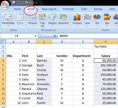
Open a blank Work sheet in Microsoft Excel.

a) Click on the Windows button on the bottom left corner of your computer screen.

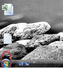
b) The Start menu pops up.

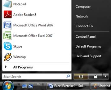
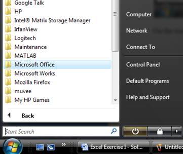
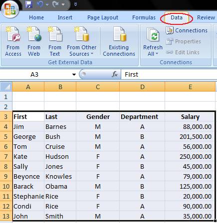
c) On the start Menu Select\ click on “All Programs”. Scroll down and select “Microsoft Office” as shown below.

d) Click on “Microsoft Office” which would give you the details of the programs available in the Microsoft Office Suite as shown below.

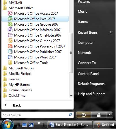
e) Scroll down and click on “Microsoft Office Excel 2007” which would open up a new Excel worksheet.

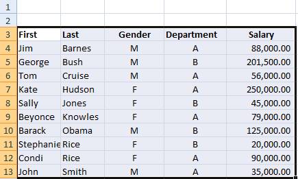
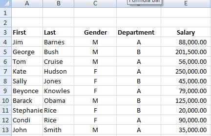
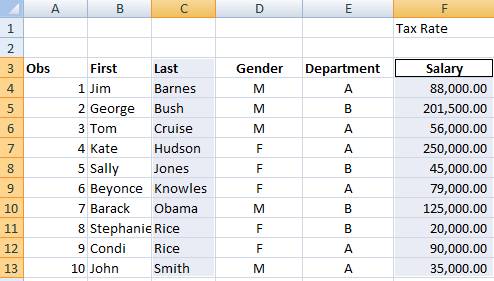
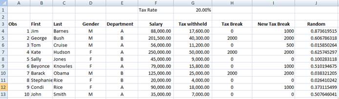
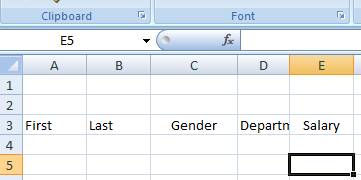
Enter the First name, Last Name, Gender, Department, And Yearly Salary (with 2 decimals) for 10 fictitious people in Columns A-E, beginning in Row 4. Be sure to enter column headings (Row 3) and align them with the data. Adjust column widths as needed.

a) First enter the column headings in Row 3 so that we can enter the data easily in an orderly manner.

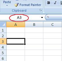
b) Select the first cell in Row 3 by clicking on the cell adjacent to 3 (Row number) under the column A. The selected cell will have a thick black border and just above the column name A excel will also show the cell we have selected as shown in the screenshot below.

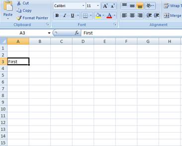
c) Keeping the cell A3 selected write down the first column label i.e. “First” in short for first name.

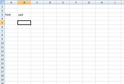
d) Now select Column B3 by clicking on the cell adjacent to cell A3 and write down the second column label i.e. “Last” for last name.

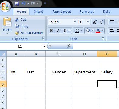
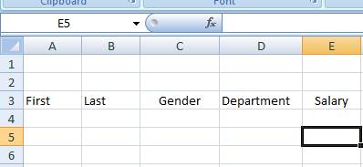
e) In a similar way enter all the column labels so that your excel worksheet looks as the screenshot shown below.

f) Sometimes a column can be small for the text inside it and the entire text may not be visible for the reader as shown below. Eg: the Department

g)

h) In such a case the width of the column can be adjusted so that the whole text is visible. To adjust the width of a column keeps your mouse pointer on the border of the column on the row having the column names say column F in our case. Once you keep the mouse pointer on the line between column F and G on the top most row the mouse pointer changes its shape with to a solid black vertical bar with tow arrows pointing to the either side.

i) Once the mouse pointer has changed its shape you can click and hold your left mouse button and drag the mouse to increase the width of the column.

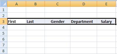
j) Now to make the column labels look different from the data select all the column labels by selecting the first column label by clicking A3, holding down the mouse button and dragging the mouse pointer over cells A3 to H3. Once you have selected the column labels it would look as in the screenshot shown below.

k) After selecting all the labels to make the labels bold click on the “B”. The column labels would look as shown below.

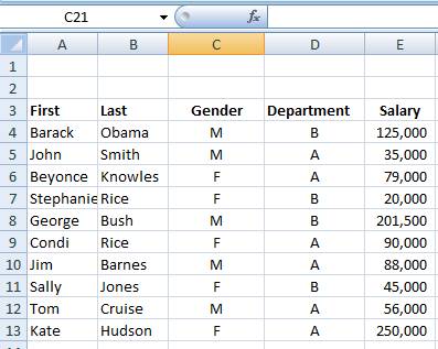
l) Now start entering the details of 10 fictitious people in the relevant columns. After entering the details your work sheet should look similar to the screenshot shown below.

j) To ensure that the yearly salary has at least 2 decimal places select the cells E4 to E13.

k) Right click on the selection to get the options menu as shown below.

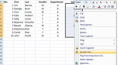
m) Click on the option “Format Cells” to open up the pop up window shown below.

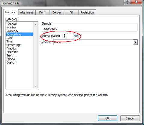
n) Select Category as accounting and click the up arrow on the decimal places box twice to ensure there are two decimal places in the salary figures. Click OK.

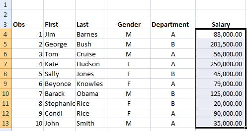
o) The Salary column would look like as shown below.

2) Sort the data by Last Name.

a) Select the whole set of the data entered by clicking cell A3 and dragging the mouse pointer to cell A13 holding down the left mouse button. By This you would select all the data entered in the first column as shown below.

b) Now to select the rest of the data, holding down the left mouse button drag the mouse pointer to cell E13 (the last entry in the salary column).

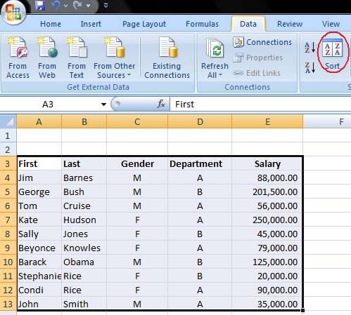
c) To sort the data by the last name select the “Data” tab.

d) After getting to the data tab click on the sort button.

e) Clicking on the sort button opens up a pop up window as shown below.

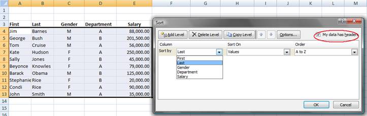
f) Ensure that “My data has headers” option is checked in the pop up and since we have to sort by the last name in the “Sort By” field select “Last” which is our column label for the last name. Click “OK”.

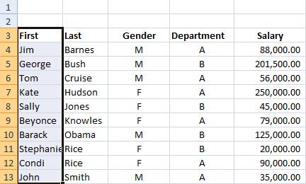
g) Once the data is sorted by the last name it should look as shown below.

3 .Insert a column before the name (new column A), and enter the Observation Number. Type only the first two numbers, then select both, and copy down for autofill.

a) To insert a column before the name column select the name column by clicking the column name “A” as shown below.

b) Click the right button of the mouse to bring up the options menu and select “Insert”

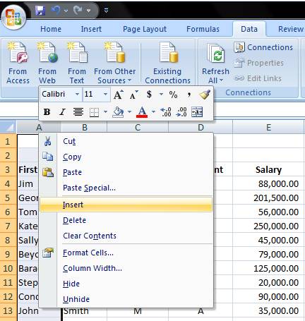
c) A new column will be inserted besides the “First” column as shown below.

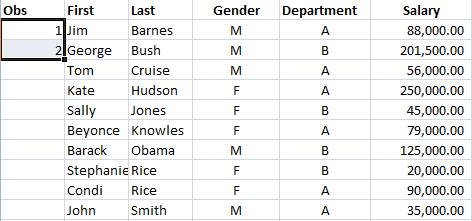
d) Give an appropriate name say “Obs” to the column and make it bold like other column headers.

e) Since Jim Barnes is our first observation write 1 besides Jim and 2 besides George Bush.

f) Select column A4 with the 1 in it. Note the black square at the bottom right of the selected cell A4 as shown below.

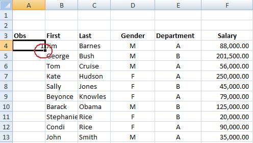
g) The solid black square is called the “Fill Handle”. Keeping A4 selected hold down the “Shift” key on your key board and press the down arrow to select cell A5 with the 2 also as shown below.

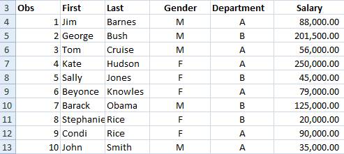
h) Keep the mouse pointer on the fill handle and once the mouse pointer changes to a black cross click the left mouse button and drag your selection to cell A13 so as to fill cells from A4 to A13 with numbers from 1-10 as shown below.

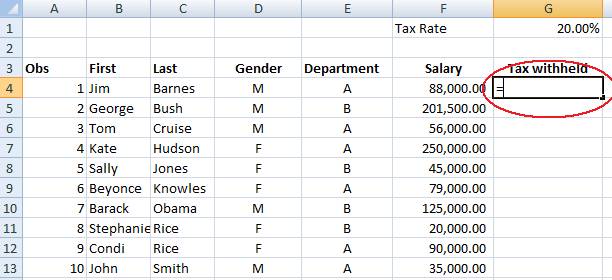
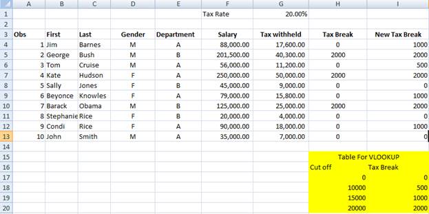
4. In Column G, type the heading “Tax Withheld”, and enter a formula that computes it. Assume 20% of the salary is withheld for taxes.

a) Enter the tax rate of 0.2 in cell G1.

b) Right click on the cell G1 to open op the options menu. Select the “Format Cells” option to bring up the dialogue box as shown below.

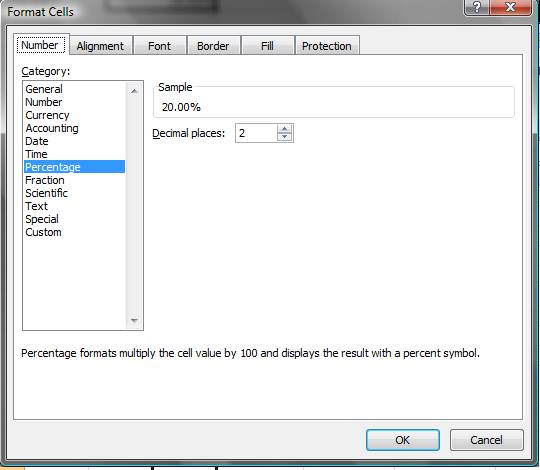
Select the category as “Percentage” and excel will automatically convert the 0.2 in cell G1 to 20%.

c) Give a column label “Tax withheld” in the cell G3.

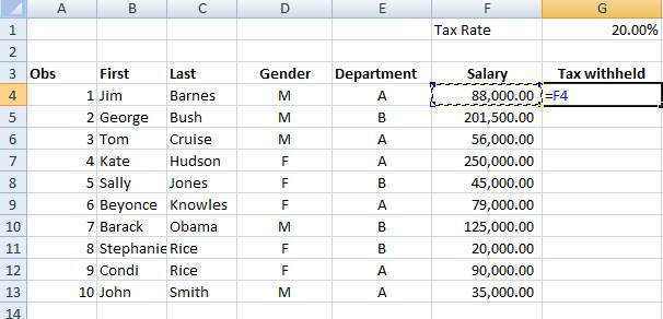
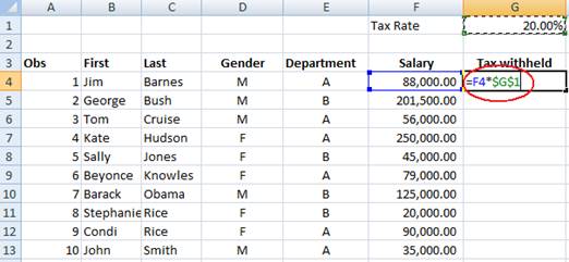
d) The tax withheld would be salary*tax rate. The tax rate is given in the cell G1. So the tax for the first person i.e. Jim Barnes can be calculated as salary of Jim Barnes (cell F4) multiplied by the tax rate (cell G1).

e) So to calculate the tax withheld select cell G4, hit the “=” key.

f) Select the cell F4 with the mouse.

g) Hit the “ * ” key

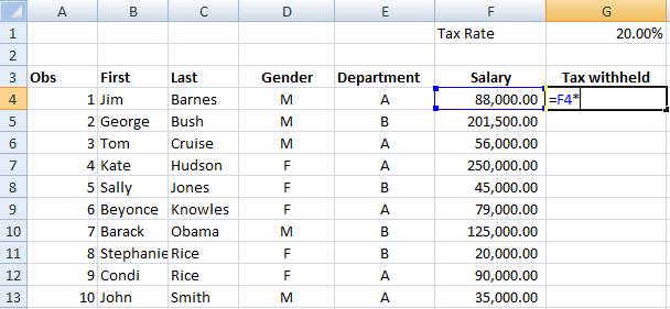
h) Now select the cell G1 i.e. the tax rate

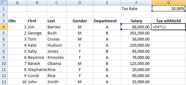
i) Since all the tax computations would refer to the cell G1 for tax rate we must freeze the cell reference to G1 in the formula. In order to do that, after selecting cell G1 hit the F4 function key. The reference to G1 will change to $G$1 as shown below

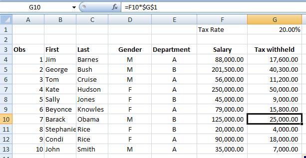
j) In order to calculate the taxes for the other 9 people we can use excel’s autofill feature.

k) Click on the fill handle for the cell G4 and drag down to cell G 13 to compute the taxes for all the other people. The sheet should look like the one shown below

5. The new tax code gives a Tax Break of $2,000 for all those who have more than $20,000 withheld. Use an IF statement to compute this in Column H.

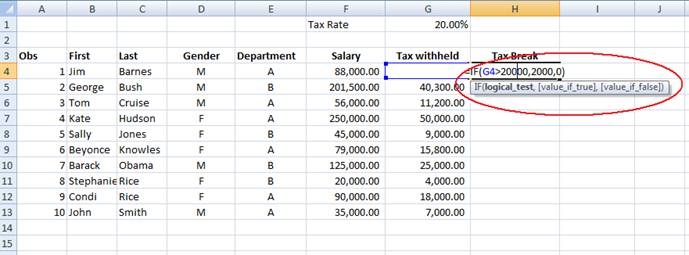
a) Assign a column header “Tax Break” in cell H3.

b) Select cell H4 and hit the “=” key.

c) After = write the formula to check if the person is eligible for a tax break or not i.e. check if he/she has paid taxes above 20000. The formula is shown in the screenshot below.

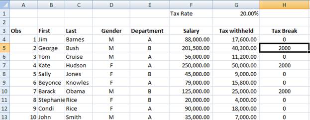
d) We can again use excels autofill function to calculate the tax breaks for the rest of the people by clicking and dragging the fill handle of the cell H4. The worksheet with all the tax break information would look like the one shown below.

6 .Assume now that the Tax Break is more complex. If you had at least $10,000 withheld, you get $500 back. If you had at least $15,000 withheld, you get $1,000 back. If you had $20,000 or more withheld, you get $2,000 back as before. Use a VLOOKUP statement to compute the New Tax Break in Column I.

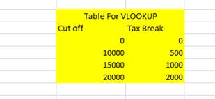
a) First step is to make the VLOOKUP table.

b) From row 15 onwards in columns H and I create a VLOOKUP table as shown in the screenshot below.

c) The VLOOKUP table is highlighted by selecting the relevant rows and columns and clicking on the color fill button in the home tab as shown below.

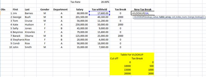
d) To find out the new tax breaks label the cell I3 as new Tax break.

e) To find out the new tax break each person’s tax payment should be compared to the taxable levels in the VLOOKUP table using the VLOOKUP command.

f) In order to compare the tax paid by the first person to the VLOOKUP table select the cell I4 and hit the “=” key.

g) After the = sign write VLOOKUP (or write VL and hit the TAB key).

h) The first input to the VLOOKUP command is the taxes paid by the individual i.e. cell G4 in this case thus select cell G4 and then the “,” key to separate the value from the other inputs we are going to give.

i) Now the taxes need to be compared to the new tax break levels which are in the VLOOKUP table. Select the new tax break data in the VLOOKUP table by selecting cells H17 through I20 as shown below.

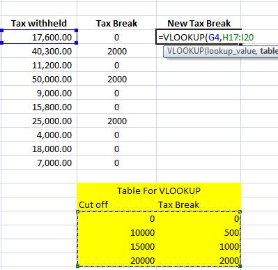
j) Since we will be referring to the same VLOOKUP table to compute all the tax breaks it would be a good idea to freeze the table by hitting the F4 function key. And also mention the range_lookup as 2. The results are shown below.

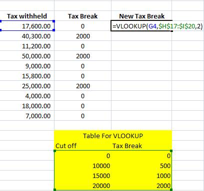
k) Once the tax break for the first person is calculated the rest can be calculated using the excels autofill function by clicking and dragging the fill handle. The final results obtained are shown below.

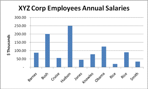
8. Draw a bar graph showing the salaries for each person, along with their last name. Label axes appropriately.

a) To draw a bar graph showing the salaries for each person, along with their last name first select cells C3 through C13.

b) Now Hold the “CTRL” key down and select cells F3 to F14 as shown below.

c) Go to the “Insert” tab.

e) Select the column option to get a chart as shown below.

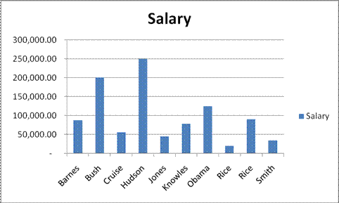
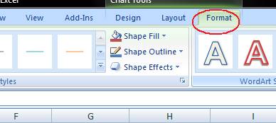
f) Select the format tab as shown.

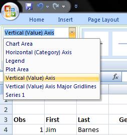
g) Go to the Current selection group on the top left and select vertical value axis as shown below.

h) Click on the “Format selection” in the current selection group to bring up the below pop up.

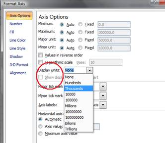
i) Change the display units to thousands and edit the title by right clicking on the title and selecting edit text. The final result is shown below.

8. You wish to choose 5 people out of the 10 at random to go shopping for a holiday party. Generate random numbers in Column J. Sort the entire dataset by the random numbers in ascending order, and Highlight the top 5 names.

a) To generate random numbers we use the rand () function.

b) Select Column J4 on the work sheet and hit the “=” key.

c) Now write “RAND ()” in the cell as shown below and hit the enter key.

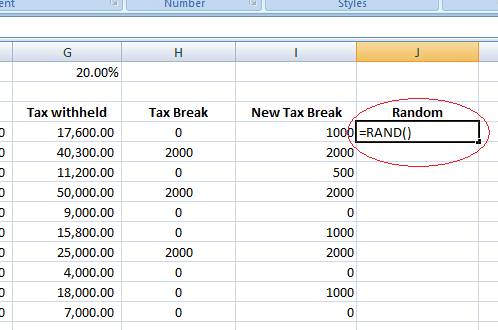
d) The cell J4 will have a random number.

e) To generate random numbers for the rest of the 9 values we can use excels autofill feature by dragging the fill handle from J4 to J13. The completed excel work sheet would look as shown below.

f) To sort the people according to the random numbers in ascending order select the column with the random numbers J4 to J13. In the home tab select Custom sort and specify “Random” as the sort by parameter.

g) Once sorted according to the random numbers select the data of the first five people and high light it with the fill color button on the home tab.